Chapter 14 Chapter 14: Network visualization in igraph
This chapter aims to introduce you the basics of network visualization. Note that for a very large network (> 100 nodes) it becomes very difficult to create good visualizations using basic igraph plotting functions. You may need to venture to other R packages (see Chapter 15 - under development). A nice open-source software for creating great network visualizations is Gephi.
14.1 Set up
We will use the karate network from Chapter 5, which contains various node and edge attributes.
library(igraph)
library(igraphdata)
library(tidyverse)

data('karate')

# import your node attributes
node_info <- read.csv('data/karate_nodes_added.csv', header = T)

# very important to ensure that node order is identical
node_info <- node_info %>% arrange(factor(node, levels = V(karate)$name))
## This graph was created by an old(er) igraph version.
## ℹ Call `igraph::upgrade_graph()` on it to use with the current igraph version.
## For now we convert it on the fly...## [1] TRUE# add the 'gender' attribute
karate <- set_vertex_attr(karate,
name = 'gender',
value = node_info$gender)
# add the 'belt' attribute
karate <- set_vertex_attr(karate,
name = 'belt',
value = node_info$belt)
# add the 'age' attribute
karate <- set_vertex_attr(karate,
name = 'age',
value = node_info$age)
# initialize all edges with the same label
E(karate)$edge_type <- 'same'
# re-assign those with mixed edges to a new label
E(karate)$edge_type[E(karate)[V(karate)[V(karate)$gender == 'male'] %--% V(karate)[V(karate)$gender == 'female']]] <- 'different'
summary(karate) # there should be a new edge type ## IGRAPH 4b458a1 UNW- 34 78 -- Zachary's karate club network
## + attr: name (g/c), Citation (g/c), Author (g/c), Faction (v/n), name (v/c), label (v/c), color (v/n), gender (v/c), belt
## | (v/c), age (v/n), weight (e/n), edge_type (e/c)14.2 Visualizing node attributes
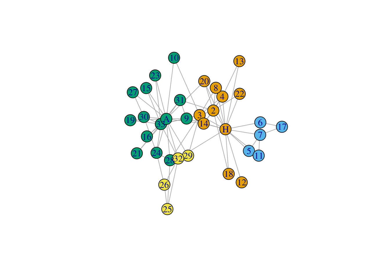
14.2.1 Color nodes by their categorical attributes
# color nodes by their attributes (categorical)
plot(karate, vertex.color = factor( V(karate)$gender )) # notice the use of factor() 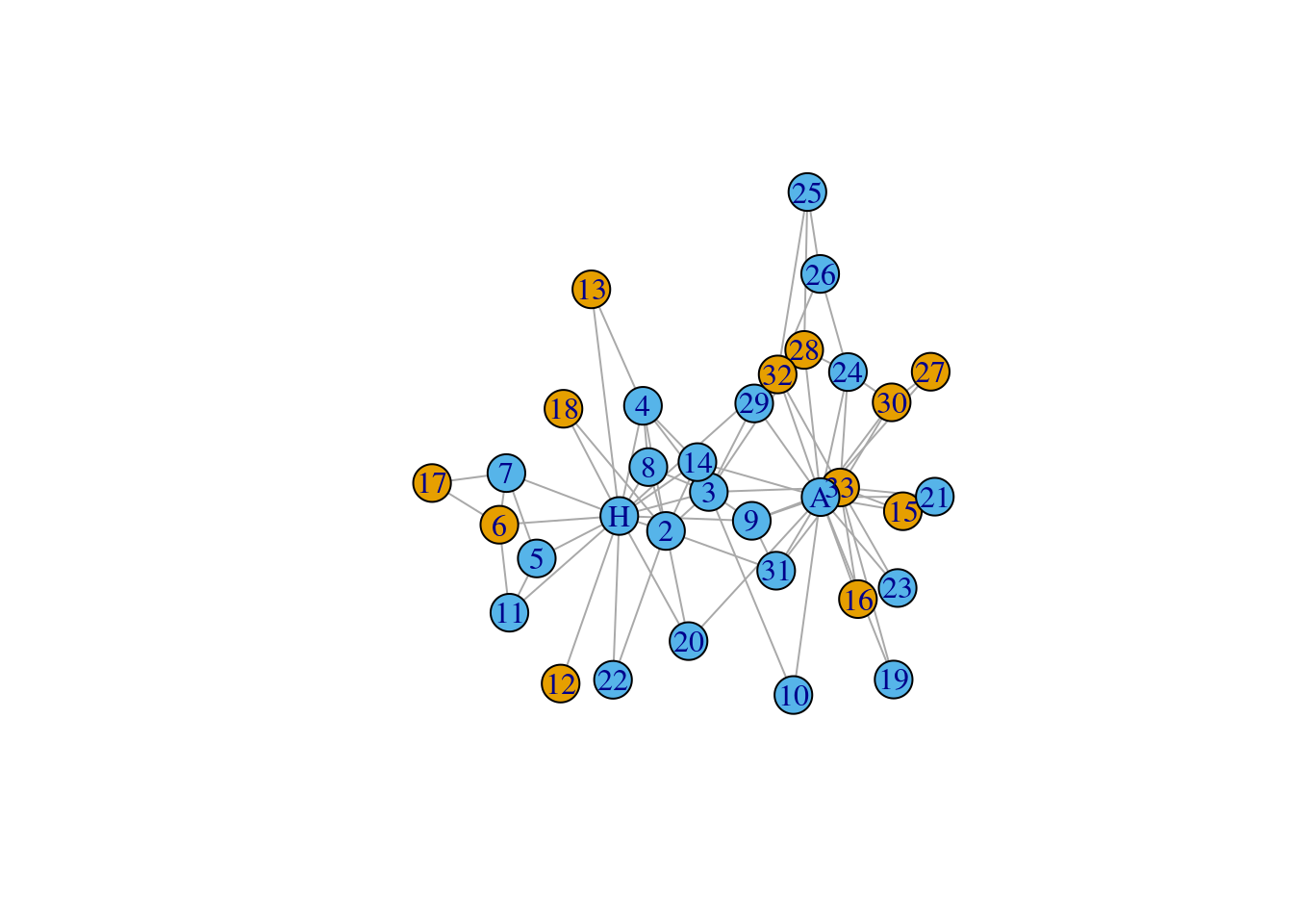
If you would like to specify your own colors, you can refer to this website for the names of colors in R and assign them to each category as shown in the following code:
## [1] "female" "male"my_colors <- c('firebrick', 'slateblue') # firebrick = female, slateblue = male
# use of square brackets to map the colors onto the labels
plot(karate, vertex.color = my_colors[ factor( V(karate)$gender ) ] ,
vertex.label.color = 'white' # to make the labels visible
)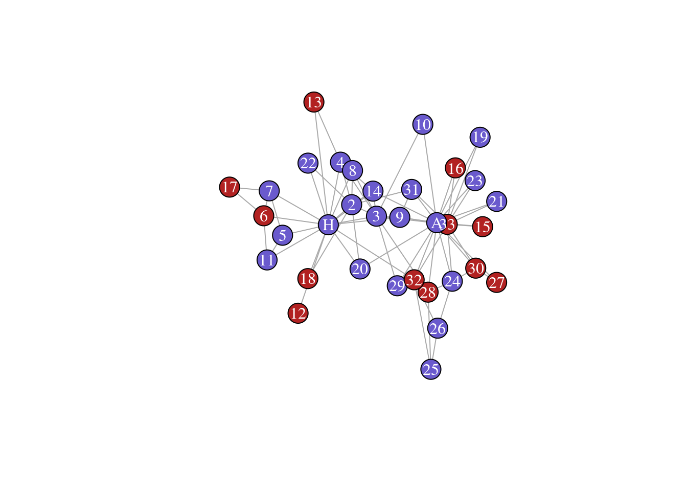
Can you try replacing the gender attribute with the belt attribute?
14.2.2 Color nodes by their continuous attributes
# color nodes by their attributes (continuous)

# a function to generate color gradients from a pre-specified palette
palf <- colorRampPalette(c("red", "green")) # smaller values = white

plot(x=10:1, y=1:10, pch=19, cex=5, col=palf(10))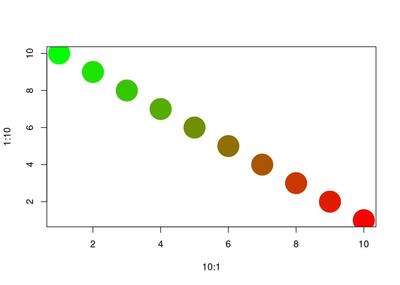
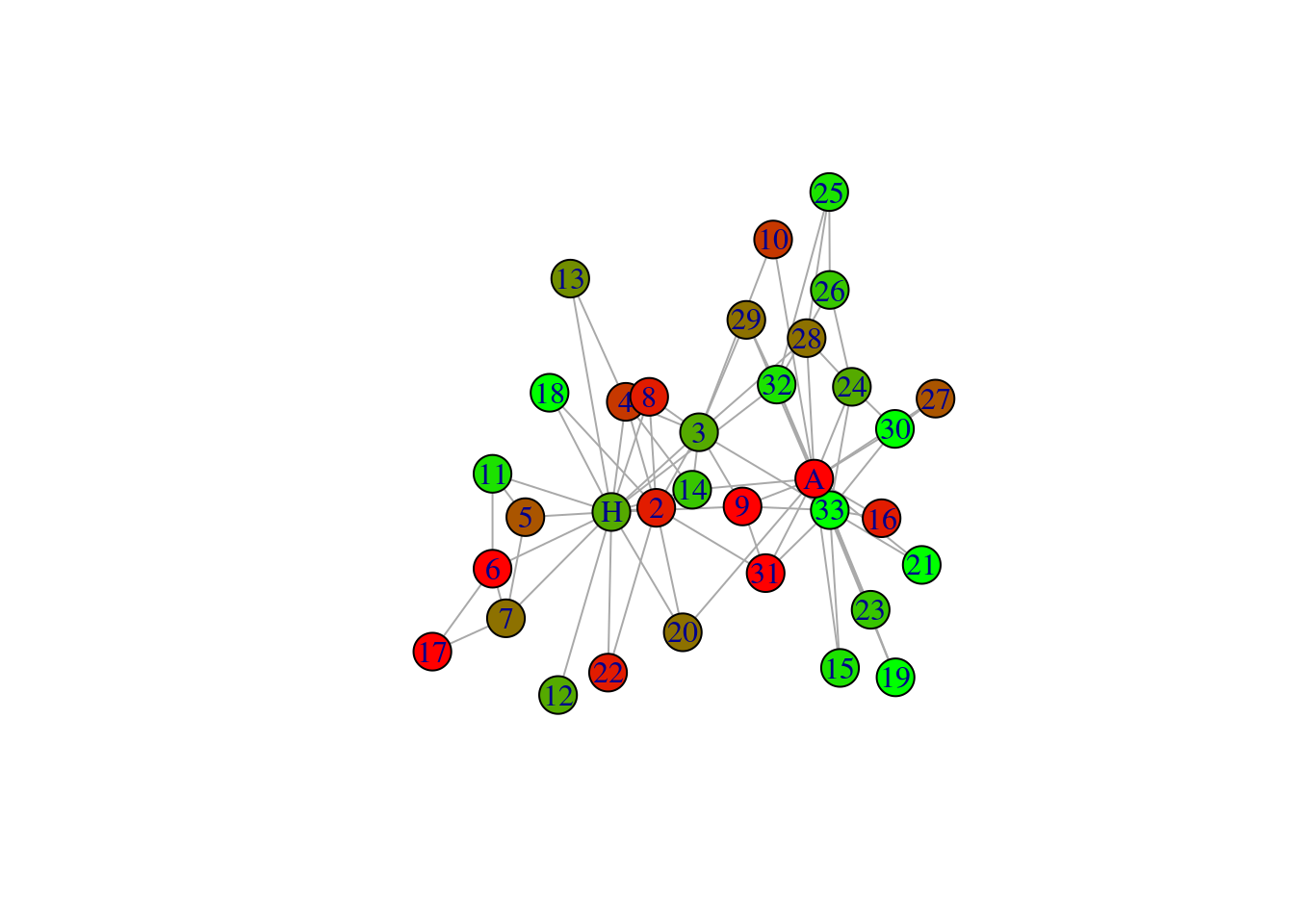
14.2.3 Node shapes by their categorical attributes
# give categorical attributes different shapes
plot(karate,
     vertex.shape = c('circle', 'square')[factor(V(karate)$gender)], # notice the use of factor() with gender to subset a vector of pre-defined node shapes
vertex.color = 'white') 
## [1] "female" "male"14.2.4 Node size by their continuous attributes
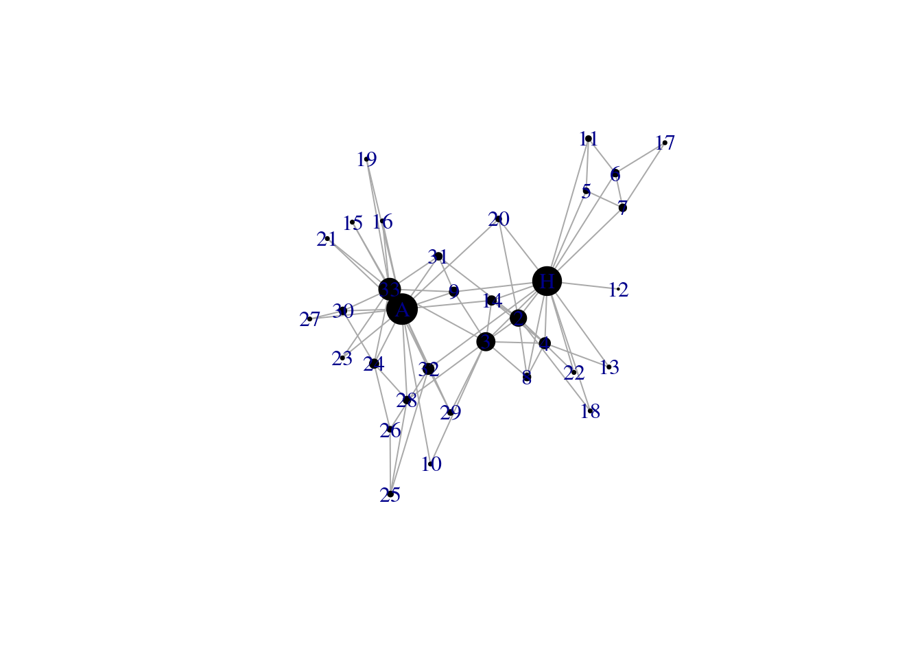
# give continuous attributes different sizes

plot(karate, vertex.size = V(karate)$age) # notice that the sizes are not very well scaled 
plot(karate, vertex.size = 0.5*V(karate)$age) # you will have to play around to find a suitable scale 
14.3 Visualizing edge attributes
14.3.1 Color edges by their categorical attributes
plot(karate, vertex.color = 'white', edge.color = factor(E(karate)$edge_type)) # note the use of factor()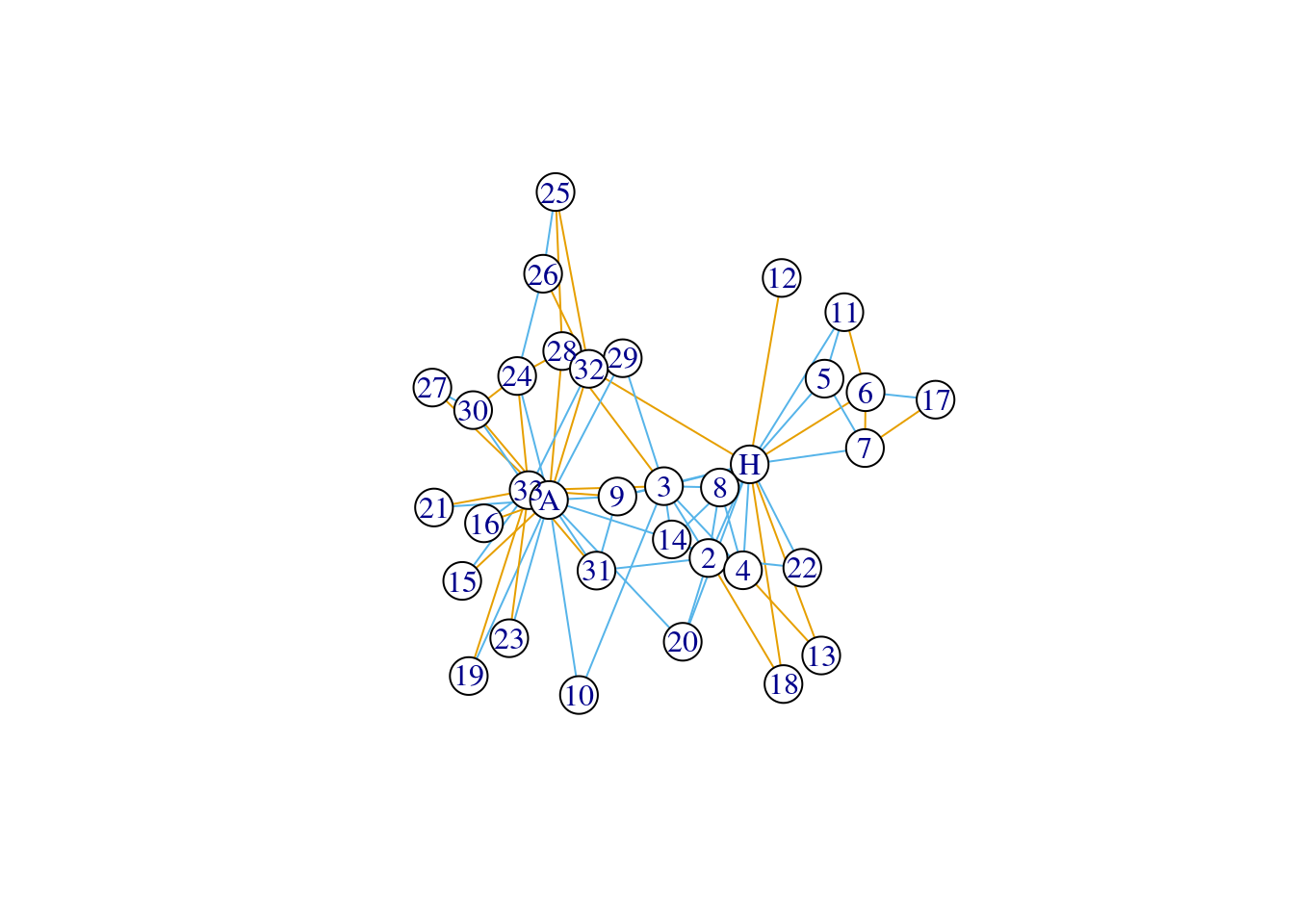
plot(karate, vertex.color = 'white', edge.color = c('red', 'blue')[factor(E(karate)$edge_type)]) # specifying your own colors 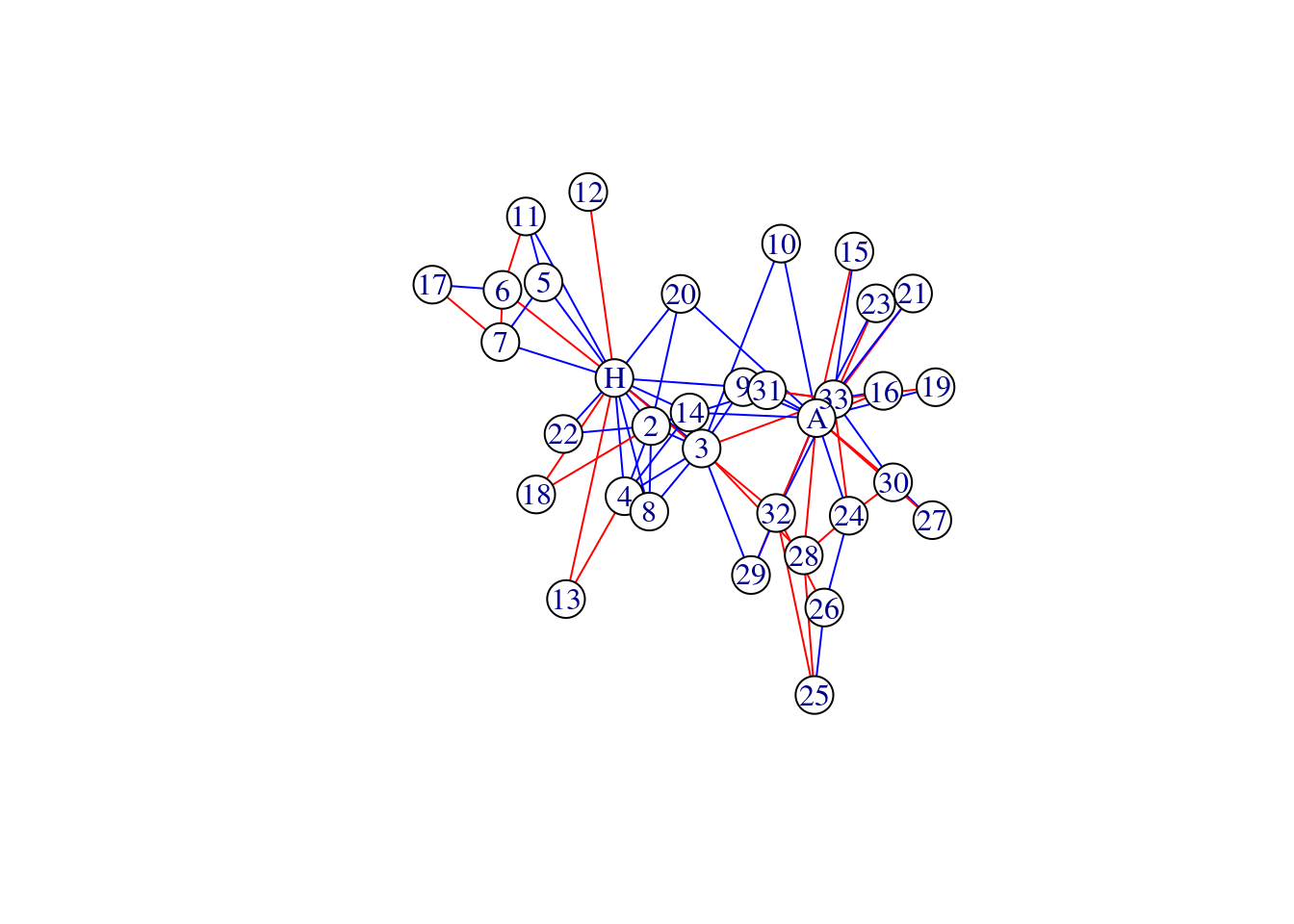
factor(E(karate)$edge_type) |> levels() # this tells you the ordering of the levels so you can tell that red = different and blue = same ## [1] "different" "same"14.4 Other
14.4.1 Graph layouts
It is good practice to set a seed before executing the graph layout functions, so that you are able to “save” the output and replicate it in the future. Notice that the layout function takes the network as its argument and outputs a 2 column matrix which is the x- and y-coordinates for each of the nodes in the network (explore the my_layout1 R object). Then you can insert that as the input to the layout parameter when you want to plot the network.
## saving a fixed layout for future use
set.seed(1)
my_layout1 <- layout_in_circle(karate)

set.seed(2)
my_layout2 <- layout_with_dh(karate)

plot(karate, layout = my_layout1)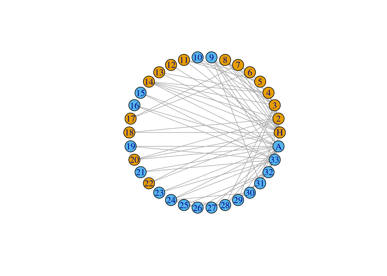
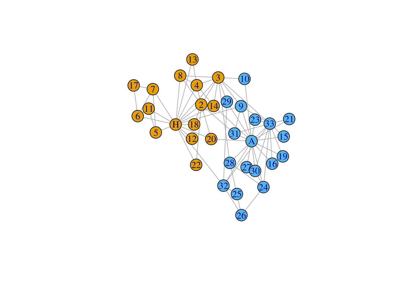
See https://kateto.net/network-visualization (Section 4.2 Network layouts) to learn more about the different plotting formats available in igraph.
14.4.2 Plot title
## add a plot title ----
plot(karate, vertex.color = V(karate)$community, main = 'Communities in the karate network')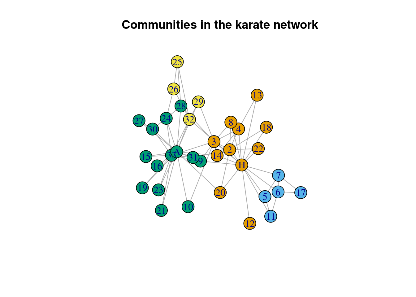
14.4.3 Add a subtitle
## add a subtitle ----
plot(karate, vertex.color = V(karate)$community, main = 'Communities in the karate network',
     sub = 'The Louvain community detection method was used.')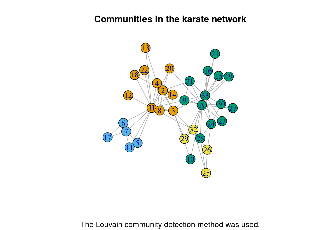
14.4.4 Multiple plots
## multiple plots ----

par(mar=c(0,0,0,0)+1, mfrow = c(1,2)) # adjust margins, 1 row, 2 columns

plot(karate, layout = my_layout1, main = 'layout 1')
plot(karate, layout = my_layout2, main = 'layout 2')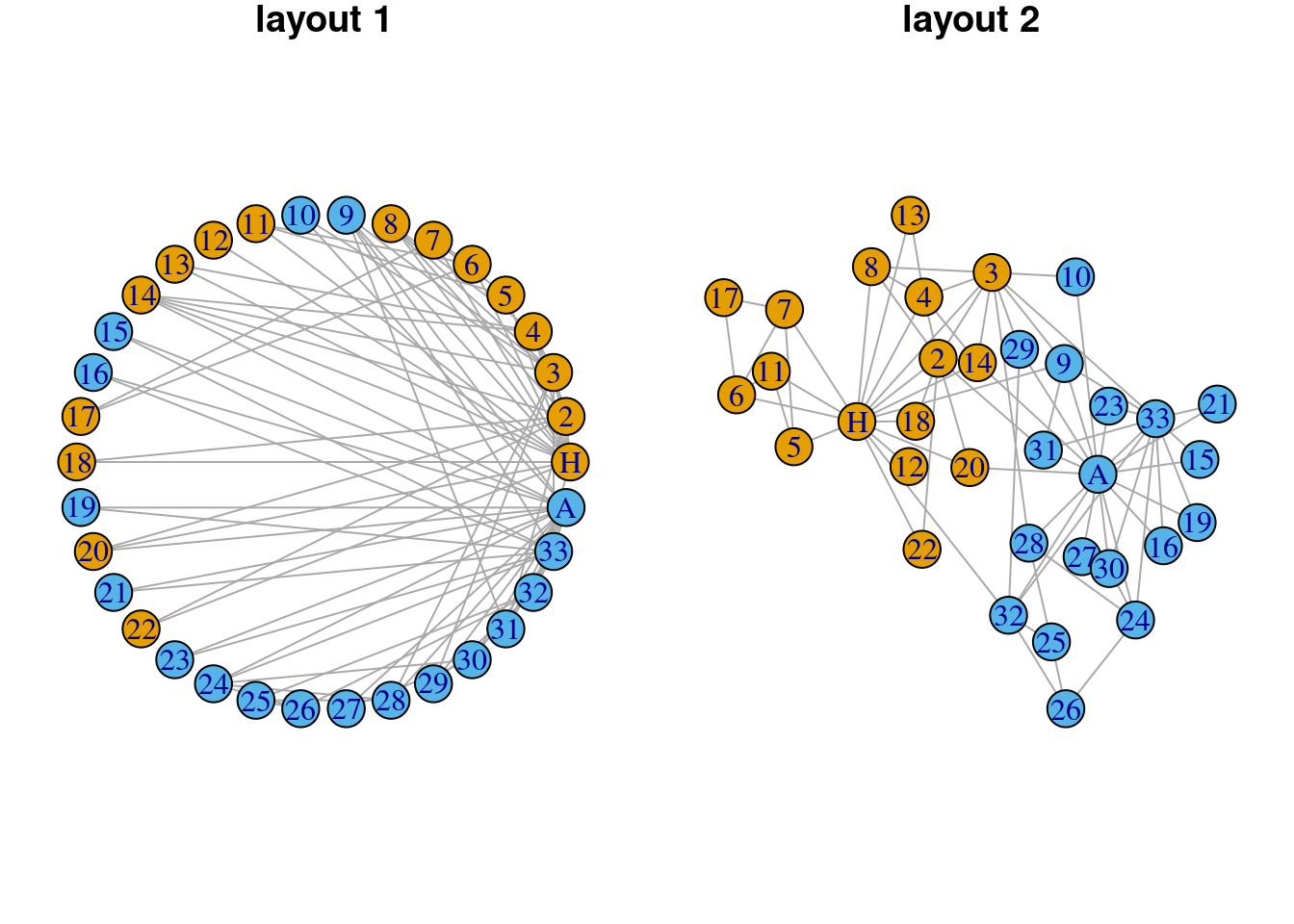
14.4.5 Useful links
Introduction to network visualization in R: https://kateto.net/network-visualization
Colors in R: https://r-charts.com/colors/
