Chapter 5 Chapter 5: Manipulating network objects
In this chapter we explore how network objects can be “manipulated” based on their node or edge attributes. This can be especially useful if you wish to segment or subset your network so that you can analyze networks of different types. For instance, you may wish to explore how your network analysis results change depending on the threshold used to remove edges of varying weights (edge attribute). Another example could be that you are only interested in analyzing language networks where the nodes represent nouns, and not other parts of speech like verbs or adjectives (node attribute). We will also learn how to add these node and edge attributes to the network.
5.1 Set up
We will use the karate network as our example in this chapter.
## This graph was created by an old(er) igraph version.
## ℹ Call `igraph::upgrade_graph()` on it to use with the current igraph version.
## For now we convert it on the fly...
## IGRAPH 4b458a1 UNW- 34 78 -- Zachary's karate club network
## + attr: name (g/c), Citation (g/c), Author (g/c), Faction (v/n), name (v/c), label (v/c), color (v/n), weight (e/n)5.2 Adding node attributes
An important feature of psychological networks is that we are usually interested in more than just the underlying mathematics of the network, but rather we want to know how these network measures relate to behavior. This implies that the nodes in psychological networks are typically associated with rich psychological variables. For instance, nodes depicting individuals of different ages and genders, or nodes depicting words with different values on lexical-semantic variables like valence and arousal.
We need to add this node information as node attributes to the network representation.
In the code below, we output the list of nodes so that we can merge this data frame to the node attributes (can be done external to RStudio or internally within RStudio using data wrangling methods). This is because node attributes are additional variables that you have knowledge of or have collected in your study.
# export your node names, enter attributes manually outside of R
write.csv(data.frame(node = V(karate)$name), file = 'karate_nodes.csv', row.names = F)
In the karate_node_added.csv file, sample node attributes for the karate network have been added. The code below shows you how to read in this data and add this information as node attributes to the network using the set_vertex_attribute function.
# import your node attributes
node_info <- read.csv('data/karate_nodes_added.csv', header = T)

# very important to ensure that node order is identical
node_info <- node_info %>% arrange(factor(node, levels = V(karate)$name))

identical(V(karate)$name, node_info$node) # sanity check that the node name order is identical
## [1] TRUE# add the 'gender' attribute
karate <- set_vertex_attr(karate,
name = 'gender',
value = node_info$gender)
# add the 'belt' attribute
karate <- set_vertex_attr(karate,
name = 'belt',
value = node_info$belt)
# add the 'age' attribute
karate <- set_vertex_attr(karate,
name = 'age',
value = node_info$age)
summary(karate) # these vertex attributes should show up in the summary## IGRAPH 4b458a1 UNW- 34 78 -- Zachary's karate club network
## + attr: name (g/c), Citation (g/c), Author (g/c), Faction (v/n), name (v/c), label (v/c), color (v/n), gender (v/c), belt
## | (v/c), age (v/n), weight (e/n)A key point is to ensure that the node ordering in your .csv file is identical to that of the network - this can be assured using the arrange function from tidyverse. This is to ensure accurate mapping from your data frame to the network.
When you run summary(karate) hopefully you will see that there are additional labels (gender, belt, age) included in the attributes section.
5.3 Adding edge attributes
Because there are usually more edges than nodes in the network, we usually do not manually insert edge attributes by hand (although it is possible!). In Chapter 4 recall that edge weights are usually included in the network at the point of network construction, as edge weights are in an additional column in the edge list that you are importing into RStudio.
Here we explore a simple case where you want to “tag” and color edges differently depending on whether the tie is between same or different genders.
# initialize all edges with the same label
E(karate)$edge_type <- 'same'

# re-assign those with mixed edges to a new label
E(karate)$edge_type[E(karate)[V(karate)[V(karate)$gender == 'male'] %--% V(karate)[V(karate)$gender == 'female']]] <- 'different'

summary(karate) # there should be a new edge type
## IGRAPH 4b458a1 UNW- 34 78 -- Zachary's karate club network
## + attr: name (g/c), Citation (g/c), Author (g/c), Faction (v/n), name (v/c), label (v/c), color (v/n), gender (v/c), belt
## | (v/c), age (v/n), weight (e/n), edge_type (e/c)## [1] "same" "same" "same" "same" "different" "same" "same" "same" "same" "different" "different"
## [12] "same" "different" "same" "same" "different" "same" "same" "same" "same" "different" "same"
## [23] "same" "same" "same" "same" "same" "same" "same" "different" "same" "different" "same"
## [34] "different" "same" "same" "same" "different" "different" "same" "different" "same" "different" "same"
## [45] "same" "same" "same" "different" "same" "different" "different" "same" "same" "different" "same"
## [56] "different" "same" "same" "different" "different" "different" "same" "same" "different" "different" "different"
## [67] "same" "different" "different" "different" "same" "same" "different" "different" "same" "same" "different"
## [78] "different"# this tells you the ordering of the levels so you can tell that red = different and blue = same
factor(E(karate)$edge_type) |> levels()## [1] "different" "same"We can then easily visualize the different edge types in the network.
# note the use of factor()
plot(karate, vertex.color = 'white', edge.color = factor(E(karate)$edge_type))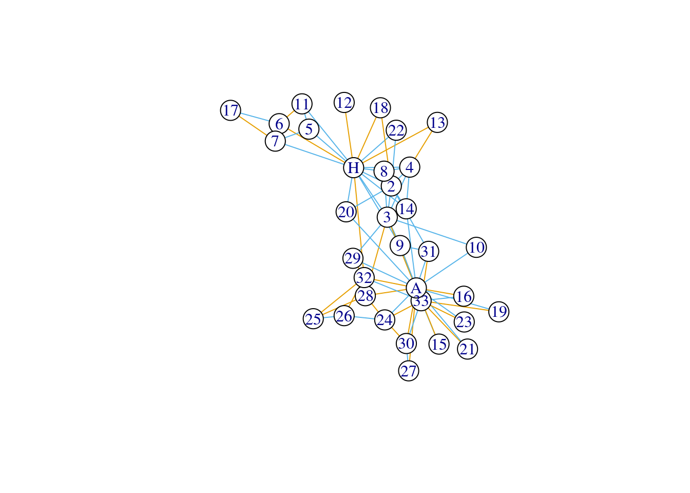
# specifying your own colors
plot(karate, vertex.color = 'white', edge.color = c('red', 'blue')[factor(E(karate)$edge_type)])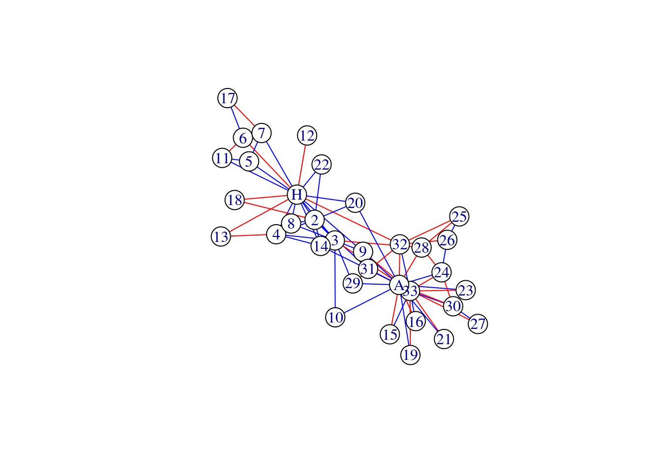
5.4 Subsetting the network
5.4.1 Subset by node attributes
The example below subsets the karate networks to only retain male individuals.
karate_male <- induced_subgraph(graph = karate,
                                vids = V(karate)$gender == 'female')

summary(karate_male)
## IGRAPH 5093168 UNW- 12 6 -- Zachary's karate club network
## + attr: name (g/c), Citation (g/c), Author (g/c), Faction (v/n), name (v/c), label (v/c), color (v/n), gender (v/c), belt
## | (v/c), age (v/n), weight (e/n), edge_type (e/c)How would you change the code to retain female individuals?
5.4.2 Subset by a target node
The example below shows you how to extract the immediate neighborhood structure of a particular node (the ego).
mrhi <- make_ego_graph(karate, order = 1, nodes = 'Actor 2')[[1]] # order = 1 (immediate neighbors)

summary(mrhi)
## IGRAPH 62c285a UNW- 10 21 -- Zachary's karate club network
## + attr: name (g/c), Citation (g/c), Author (g/c), Faction (v/n), name (v/c), label (v/c), color (v/n), gender (v/c), belt
## | (v/c), age (v/n), weight (e/n), edge_type (e/c)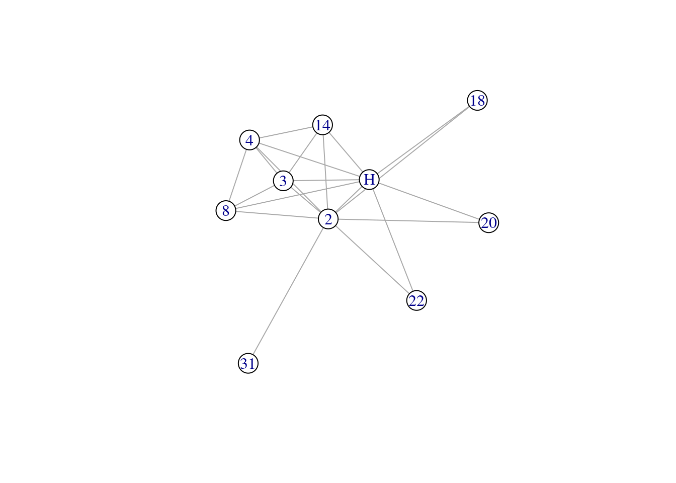
We can also extract the ego’s 2-hop neighborhood - this includes their immediate connections, and the connections of the connections. This can be easily done by changing the order argument.
mrhi2 <- make_ego_graph(karate, order = 2, nodes = 'Mr Hi')[[1]] # order = 2 (immediate + neighbors of neighbors)

summary(mrhi2)
## IGRAPH 99baf9d UNW- 26 59 -- Zachary's karate club network
## + attr: name (g/c), Citation (g/c), Author (g/c), Faction (v/n), name (v/c), label (v/c), color (v/n), gender (v/c), belt
## | (v/c), age (v/n), weight (e/n), edge_type (e/c)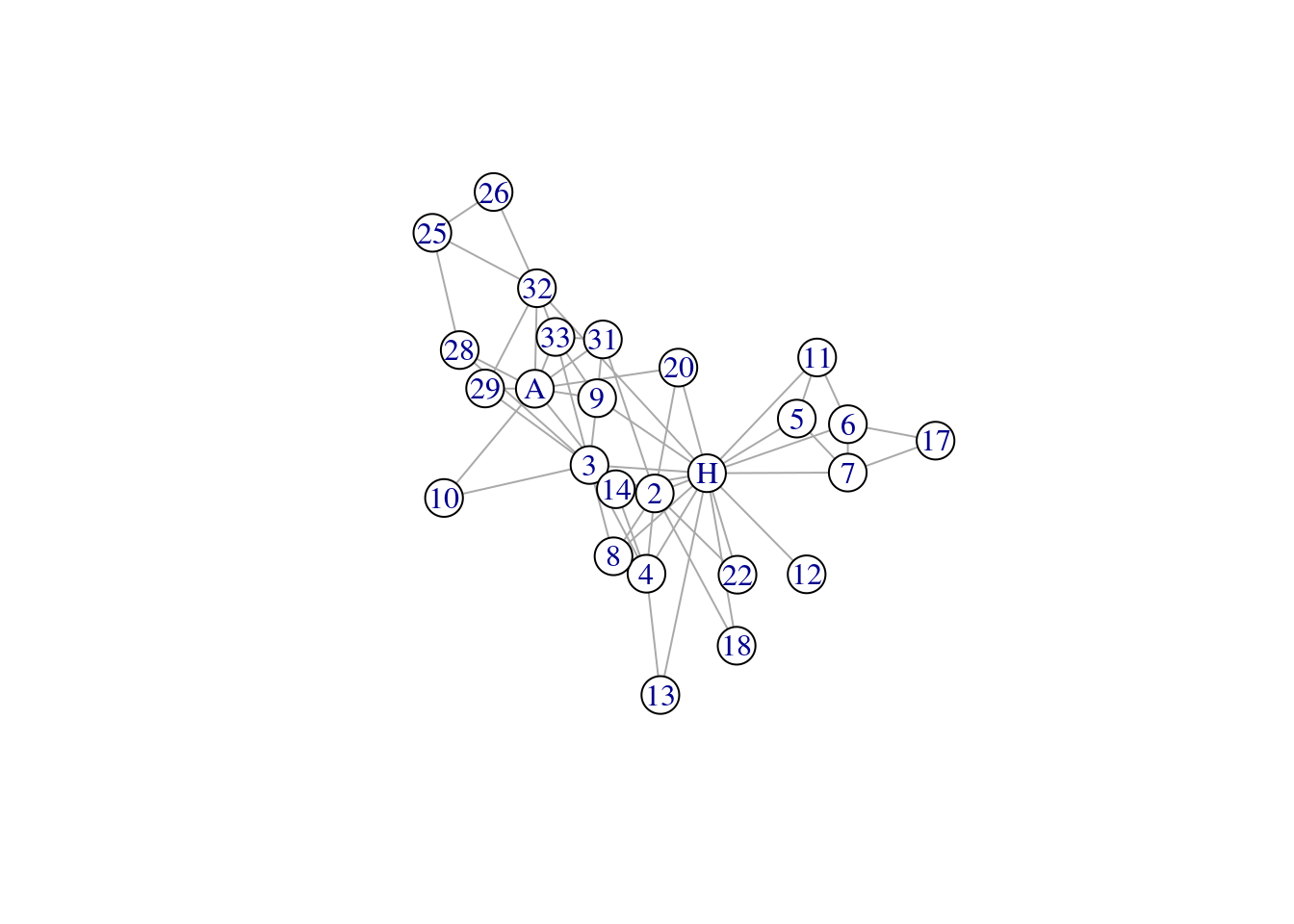
5.4.3 Subset by removing a group of nodes
The example below shows you how you can remove a set of nodes and its incident edges (John A and Mr Hi) from the karate network and save the output as a new network object. Note that you need to specify the name of the nodes as a character vector. If the network does not have named nodes, then it takes a numeric vector of numbers as the nodes to remove (i.e., the number corresponds to the node order in the network object).
karate_new <- delete_vertices(karate, v = c('John A', 'Mr Hi'))

plot(karate_new, vertex.color = 'white')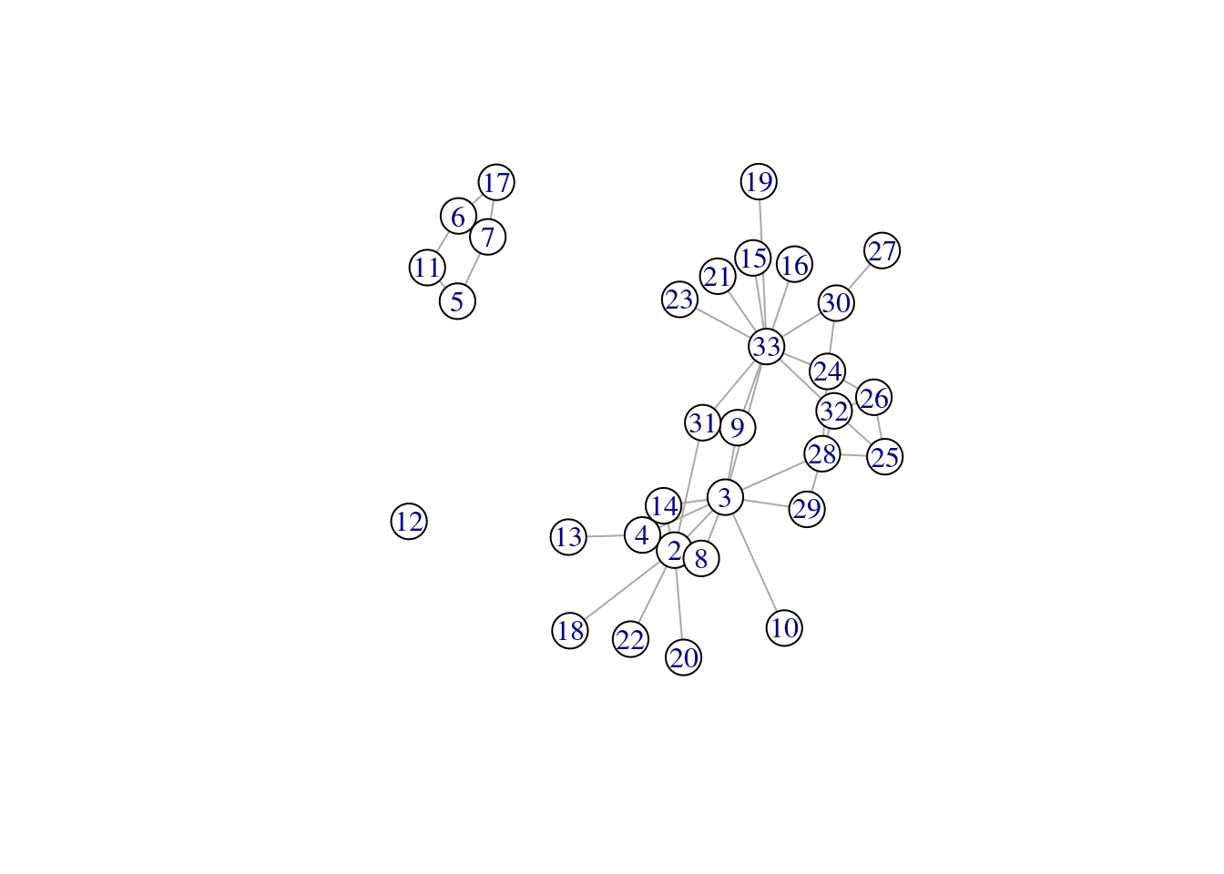
Notice how the network has fragmented into separate network components after the removal of these two nodes.
5.4.4 Subset by edge attributes
We can also subset a network by their edge attributes. Below shows an example where we only want to retain edges that between males and females (i.e., different genders).
The eids argument looks a bit crazy, but what it is doing to subset from all of the edges in the original network, the set of edges that connect nodes that are female and male. %--% is a special igraph operator that looks for the edges that join two sets of specified vertices (here we are using the square operator to select nodes of various attributes). Think about what aspect of this argument you would be modify in order to retain the edges between females only.
# retain edges of the network where the connection is between a male and a female (i.e., mixed edges)
mixed_network <- subgraph.edges(graph = karate,
                                eids = E(karate)[V(karate)[V(karate)$gender == 'female'] %--% V(karate)[V(karate)$gender == 'male']]
                                )

# eids = E(network)$weight > 4

plot(mixed_network, vertex.color = factor(V(mixed_network)$gender)) 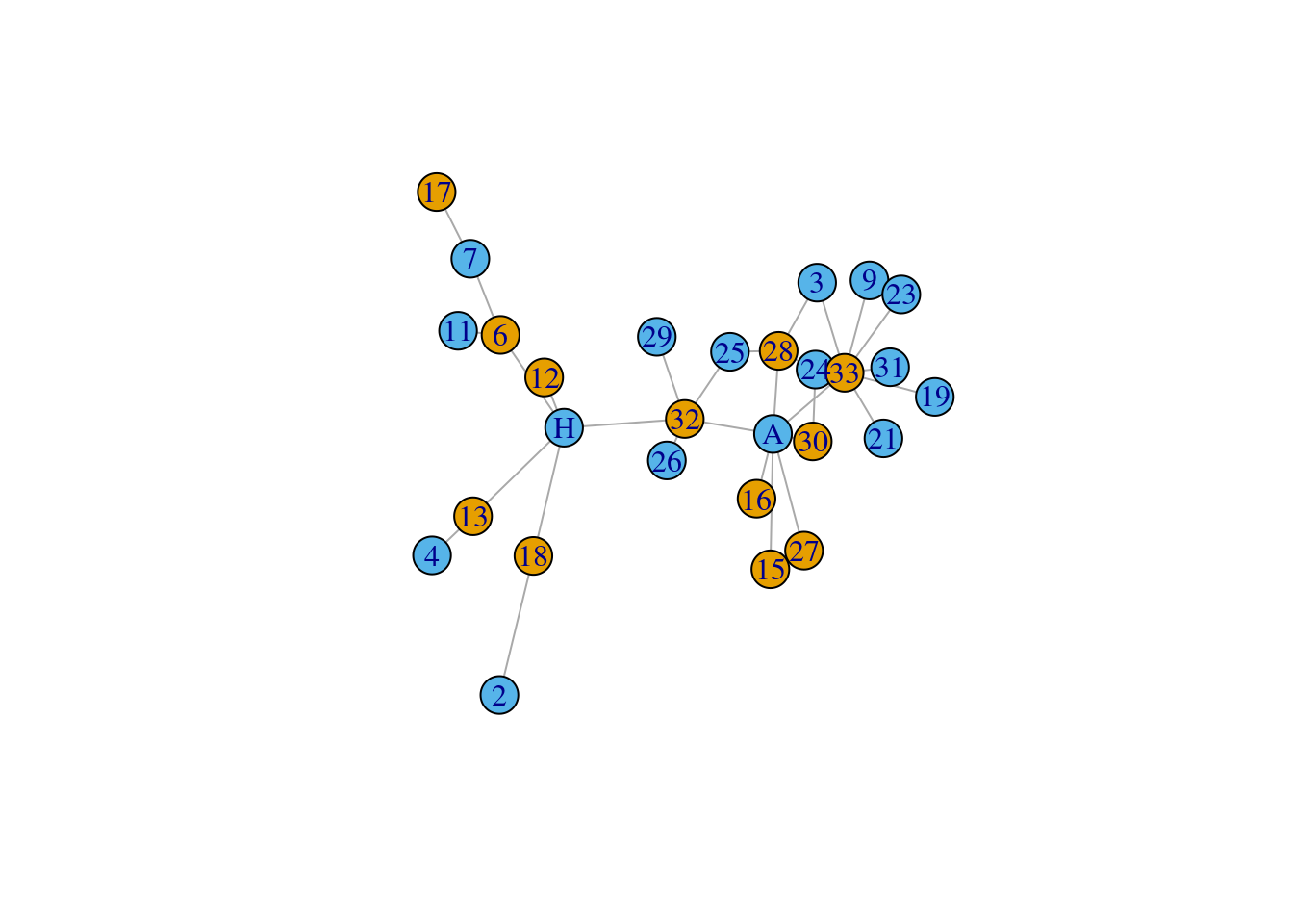
If you have a weighted graph, it is also possible to subset the network based on edge weights. The code below retains edges that have a weight greater than 4. Play around with this argument and see if you can subset the network based on different weight thresholds. For instance, if you are interested in studying acquaintance relations, then you may decide to retain weak edges, but if you are interested in studying close relations, then you may decide to retain the strongest edges.
example_network <- subgraph.edges(graph = karate,
                                  eids = E(karate)[E(karate)$weight > 4]
                                  )

plot(example_network)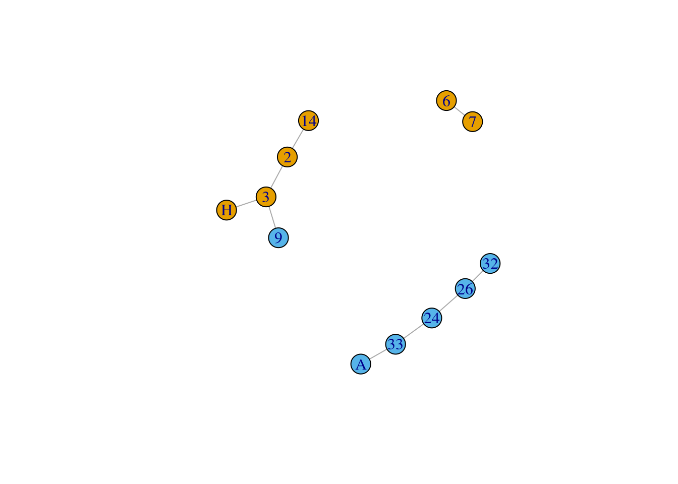
5.4.5 Subsetting by mutual edges
This section is most applicable for directed networks, as you may wish to subset a network based on whether edges are mutual (1–>2 AND 2–>1) or asymmetrical (1–>2 but there is no connection from 2 to 1).
To illustrate this, we first have to convert our karate network into a directed graph.
karate_d1 <- as.directed(karate, mode = 'random') # convert undirected edges into directed edges
karate_d2 <- as.directed(karate, mode = 'mutual') # convert undirected edges into mutual, directed edges

summary(karate_d1)
## IGRAPH 64decc5 DNW- 34 78 -- Zachary's karate club network
## + attr: name (g/c), Citation (g/c), Author (g/c), Faction (v/n), name (v/c), label (v/c), color (v/n), gender (v/c), belt
## | (v/c), age (v/n), weight (e/n), edge_type (e/c)## IGRAPH 77fa127 DNW- 34 156 -- Zachary's karate club network
## + attr: name (g/c), Citation (g/c), Author (g/c), Faction (v/n), name (v/c), label (v/c), color (v/n), gender (v/c), belt
## | (v/c), age (v/n), weight (e/n), edge_type (e/c)Notice from the summary output that karate_d2 has twice the number of edges than karate_d1. This is because each undirected edge has been converted into two directed edges (mutual) connecting the node pair in both directions.
We can use the function which_mutual to detect mutual directed edges in the network and use this to subset the network accordingly. Notice that to select for the non-mutual edges, we can use the ! or NOT operator.
# retain mutual edges
subgraph.edges(karate_d1, eids = E(karate_d1)[which_mutual(karate_d1)], delete.vertices = TRUE) |>
  summary() # empty graph
## IGRAPH f2ca65c DNW- 0 0 -- Zachary's karate club network
## + attr: name (g/c), Citation (g/c), Author (g/c), Faction (v/n), name (v/c), label (v/c), color (v/n), gender (v/c), belt
## | (v/c), age (v/n), weight (e/n), edge_type (e/c)subgraph.edges(karate_d2, eids = E(karate_d2)[which_mutual(karate_d2)], delete.vertices = TRUE) |>
summary()## IGRAPH d3dc4ff DNW- 34 156 -- Zachary's karate club network
## + attr: name (g/c), Citation (g/c), Author (g/c), Faction (v/n), name (v/c), label (v/c), color (v/n), gender (v/c), belt
## | (v/c), age (v/n), weight (e/n), edge_type (e/c)# retain non-mutual edges
subgraph.edges(karate_d1, eids = E(karate_d1)[!which_mutual(karate_d1)], delete.vertices = TRUE) |>
summary()## IGRAPH 5d6f3d4 DNW- 34 78 -- Zachary's karate club network
## + attr: name (g/c), Citation (g/c), Author (g/c), Faction (v/n), name (v/c), label (v/c), color (v/n), gender (v/c), belt
## | (v/c), age (v/n), weight (e/n), edge_type (e/c)subgraph.edges(karate_d2, eids = E(karate_d2)[!which_mutual(karate_d2)], delete.vertices = TRUE) |>
summary() # empty graph## IGRAPH ba48d6c DNW- 0 0 -- Zachary's karate club network
## + attr: name (g/c), Citation (g/c), Author (g/c), Faction (v/n), name (v/c), label (v/c), color (v/n), gender (v/c), belt
## | (v/c), age (v/n), weight (e/n), edge_type (e/c)Notice from the summary output that you get different results depending on the way that the directed graph is constructed. In these toy examples, the directed edges in the network were either ALL mutual edges or ALL non-mutual edges. If you have a network with varying proportions of mutual and non-mutual edges these functions can be useful for assessing the overall mutuality of the directed graph.
5.5 Useful functions
Finally, below are some useful functions for network manipulations that you can learn more about by reading the documentatoin.
5.6 Exercise
Let’s continue working on Janelle’s cat interaction network you’ve created in Chapter 4.
Janelle continued observing her cats and noticed that some pairs of cats interacted more frequently with other than other pairs of cats.
Your task is to:
How would you include this extra information about the frequency of interaction into the original raw data file? (Hint: The edge list approach is beter for this, and you can put in some made up numbers from 1 to 10 to depict frequency of interaction).
Create a network object that includes this new information. (Hint: Is interaction frequency a node or edge attribute?)
Janelle has a .csv file containing the ages of the cats. How can you create a network object that includes this information? (Hint: Is cat age a node or edge attribute? Do you need to create a second file containing this information (feel free to make up some numeric data)?)
Subset the network to only show the 4 oldest cats. How many edges does this network have?
Subset the network to only show cats that interacted frequently with each other. How many nodes and edges does this network have?
Create a network visualization of the entire cat network and make at least one modification to the default plot (see Chapter 14 for ideas). For instance, can you color the nodes based on the cat’s ages?